Sound field mapping
Our services
- Sound field mapping using a sound intensity probe
- Sound field mapping using sound pressure measurement
- Localization of unwanted sound sources
- Assessment of acoustic measures on a structure
- Easy interpretation of results
Brief overview
In sound field mapping, the measured sound levels are visualized as a color gradient over a photo of the measured object, making it quickly visually recognizable at which points the measured object emits the most sound. In practice, three methods have proven successful for the creation of sound field maps. Sound field mapping by means of sound intensity measurements is carried out when a stationary acoustic problem is present. Sound intensities are measured successively at a large number of spatially well-defined positions. In practice, the positioning of the SI probe often turns out to be very time-consuming. For this reason, we have developed a software that automatically calculates these positions and displays them spatially through augmented reality glasses. Another method is acoustic near-field holography. This is mainly used when many sound sources are close to each other. However, it may also be the case that sound needs to be determined at a great distance from the sound source. For this purpose, far-field methods using beamforming are employed, which make use of acoustic cameras.
How is sound localized by sound field mapping?
Sound field mapping is a very efficient measurement method to quickly detect acoustic problem areas. A sound field map usually displays the measured sound levels as a color gradient over a photo of the measured structure. This superimposed representation allows the acoustic trouble areas to be quickly identified. In the broadest sense, this representation is comparable to contour lines on maps.
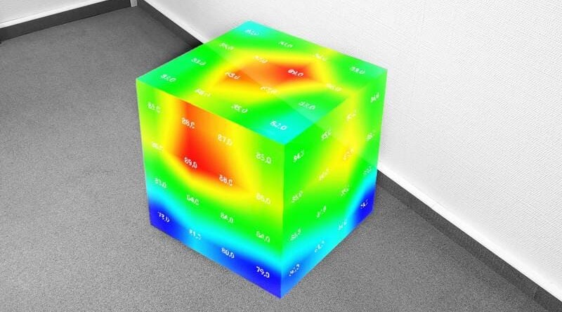
To create such maps, acoustic measurements must be performed at a large number of spatially precisely defined positions. Subsequently, the interpolation between the measuring points is performed using various mathematical methods. The following figure shows an exemplary sound field map over a PC workstation with 2 loudspeakers (for better clarification only over the right side). From this map, it can be quickly seen that most of the noise comes from the loudspeaker.
There are two major problems with conventional sound field mapping. On the one hand, the measurement of the spatially precisely defined measurement positions is very time-consuming and, on the other hand, only a two-dimensional representation of the sound field map over a photo of the measurement object is possible. For this reason, we have developed software that automatically calculates the measurement positions and displays them through augmented reality glasses. After entering the measurement results, the sound field map is also automatically calculated and virtually superimposed over the measurement object. Due to the three-dimensional display, the operator can now walk around the measurement object and see exactly where problem areas occur. The following graphic shows the differences between a conventional two-dimensional representation (left) and the three-dimensional representation using augmented reality (right).

What are the different measurement methods?
In practice, there are three different methods for sound field mapping.
Sound field mapping by using sound intensity measurements
If a stationary acoustic problem is present, the use of sound field mapping by means of a sound intensity probe is suitable. The sound intensities are measured successively at the defined positions. A corresponding software then graphically superimposes the measurement results on an image, allowing the radiated sound power on this partial area to be determined. Furthermore, it is possible to precisely quantify changes in the structure with a new measurement. The results can then be used to derive and evaluate various measures.
This method for sound field mapping imposes relatively low requirements on the measurement technology, since it requires only two channels and an SI probe. On the other hand, however, the effort required to carry it out is somewhat higher.
Our patented augmented reality solution provides the exact measurement positions virtually through AR glasses. This shortens the execution of such a sound field mapping by up to 80%.
Feel free to send us a message if you are interested in this method. We will be happy to help you.
Acoustic near-field holography
For some measurement objects, it may occur that a large number of potential sound sources are present in a very confined space (e.g. in the case of a combustion engine). To ensure reliable localization of these sound sources, a very high spatial resolution is required. In practice, a sound pressure microphone array is used for this purpose. These arrays, which are usually hand-held, are moved several times at a distance of 10-15 cm above the surface of the test object. The small distance is necessary for them to operate in the near acoustic field of the object.
The significant advantage of this method is that even closely spaced sound sources can be reliably separated and ordered. However, the requirements for the measuring equipment are considerably higher (= higher costs) than for sound field mapping by using sound intensity measurements.
Far-field methods using beamforming
The far-field methods also work with a microphone array. However, the sound sources are determined using the effect of the time-of-flight difference at a great distance from the sound source. This is done using beamforming calculations (method for determining the position of sources in wave fields).
In practice, the far-field method is performed using so-called acoustic cameras. Such systems are very well suited to quickly detect acoustic problem areas. However, additional measurement equipment is also required here. In addition, measures for improvement are difficult to quantify with a renewed comparative measurement.
If you are undecided which of these methods you should choose in your specific case, we will be happy to advise you. We also offer to map the sound field of your measurement object for you.
SOUND FIELD MAPPING
Our services
- Sound field mapping using a sound intensity probe
- Sound field mapping using sound pressure measurement
- Localization of unwanted sound sources
- Assessment of acoustic measures on a structure
- Easy interpretation of results
Brief overview
In sound field mapping, the measured sound levels are visualized as a color gradient over a photo of the measured object, making it quickly visually recognizable at which points the measured object emits the most sound. In practice, three methods have proven successful for the creation of sound field maps. Sound field mapping by means of sound intensity measurements is carried out when a stationary acoustic problem is present. Sound intensities are measured successively at a large number of spatially well-defined positions. In practice, the positioning of the SI probe often turns out to be very time-consuming. For this reason, we have developed a software that automatically calculates these positions and displays them spatially through augmented reality glasses. Another method is acoustic near-field holography. This is mainly used when many sound sources are close to each other. However, it may also be the case that sound needs to be determined at a great distance from the sound source. For this purpose, far-field methods using beamforming are employed, which make use of acoustic cameras.
How is sound localized by sound field mapping?
Sound field mapping is a very efficient measurement method to quickly detect acoustic problem areas. A sound field map usually displays the measured sound levels as a color gradient over a photo of the measured structure. This superimposed representation allows the acoustic trouble areas to be quickly identified. In the broadest sense, this representation is comparable to contour lines on maps.
To create such maps, acoustic measurements must be performed at a large number of spatially precisely defined positions. Subsequently, the interpolation between the measuring points is performed using various mathematical methods. The following figure shows an exemplary sound field map over a PC workstation with 2 loudspeakers (for better clarification only over the right side). From this map, it can be quickly seen that most of the noise comes from the loudspeaker.
There are two major problems with conventional sound field mapping. On the one hand, the measurement of the spatially precisely defined measurement positions is very time-consuming and, on the other hand, only a two-dimensional representation of the sound field map over a photo of the measurement object is possible. For this reason, we have developed software that automatically calculates the measurement positions and displays them through augmented reality glasses. After entering the measurement results, the sound field map is also automatically calculated and virtually superimposed over the measurement object. Due to the three-dimensional display, the operator can now walk around the measurement object and see exactly where problem areas occur. The following graphic shows the differences between a conventional two-dimensional representation (left) and the three-dimensional representation using augmented reality (right).
What are the different measurement methods?
In practice, there are three different methods for sound field mapping.
Sound field mapping by using sound intensity measurements
If a stationary acoustic problem is present, the use of sound field mapping by means of a sound intensity probe is suitable. The sound intensities are measured successively at the defined positions. A corresponding software then graphically superimposes the measurement results on an image, allowing the radiated sound power on this partial area to be determined. Furthermore, it is possible to precisely quantify changes in the structure with a new measurement. The results can then be used to derive and evaluate various measures.
This method for sound field mapping imposes relatively low requirements on the measurement technology, since it requires only two channels and an SI probe. On the other hand, however, the effort required to carry it out is somewhat higher.
Our patented augmented reality solution provides the exact measurement positions virtually through AR glasses. This shortens the execution of such a sound field mapping by up to 80%.
Feel free to send us a message if you are interested in this method. We will be happy to help you.
Acoustic near-field holography
For some measurement objects, it may occur that a large number of potential sound sources are present in a very confined space (e.g. in the case of a combustion engine). To ensure reliable localization of these sound sources, a very high spatial resolution is required. In practice, a sound pressure microphone array is used for this purpose. These arrays, which are usually hand-held, are moved several times at a distance of 10-15 cm above the surface of the test object. The small distance is necessary for them to operate in the near acoustic field of the object.
The significant advantage of this method is that even closely spaced sound sources can be reliably separated and ordered. However, the requirements for the measuring equipment are considerably higher (= higher costs) than for sound field mapping by using sound intensity measurements.
Far-field methods using beamforming
The far-field methods also work with a microphone array. However, the sound sources are determined using the effect of the time-of-flight difference at a great distance from the sound source. This is done using beamforming calculations (method for determining the position of sources in wave fields).
In practice, the far-field method is performed using so-called acoustic cameras. Such systems are very well suited to quickly detect acoustic problem areas. However, additional measurement equipment is also required here. In addition, measures for improvement are difficult to quantify with a renewed comparative measurement.
If you are undecided which of these methods you should choose in your specific case, we will be happy to advise you. We also offer to map the sound field of your measurement object for you.